Microsoft Research: Advancing science and technology to benefit humanity
MICROSOFT RESEARCH PODCAST
Abstracts: April 16, 2024

Microsoft Research Blog
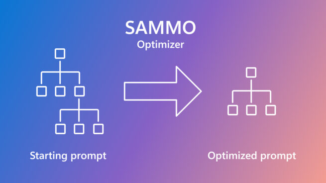
SAMMO: A general-purpose framework for prompt optimization
April 18, 2024 | Tobias Schnabel, Jennifer Neville

Microsoft Research Blog
Microsoft at NSDI 2024: Discoveries and implementations in networked systems
April 16, 2024 | Ranveer Chandra