Microsoft Research The AI Revolution in Medicine, Revisited A Microsoft Research Podcast series Learn more Featured Podcasts Apr 3 Real-world healthcare AI development and deployment—at scale Publication Video Featured Blogs Mar 26 Research Focus: Week of March 24, 2025 Publication Featured Podcasts Mar 20 The reality of generative AI in the clinic Publication Featured Videos Mar 11 Director of Microsoft Research talks AI for science (what it really means) Blogs Apr 2 VidTok introduces compact, efficient tokenization to enhance AI video processing Download Publication Publications Mar 31 Inference-Time Scaling for Complex Tasks: Where We Stand and What Lies Ahead Download Podcasts Mar 31 Ideas: Accelerating Foundation Models Research: AI for all Events Apr 26 Microsoft at CHI 2025 Publication News Mar 26 Nuclear fusion: Delivering on the promise of carbon‑free power with the help of AI Publications Mar 22 SNRAware: Improved Deep Learning MRI Denoising with SNR Unit Training and G-factor Map Augmentation News Mar 13 Jim Weinstein named among great leaders in healthcare by Becker's Hospital Review Publications May 1 Robust Optical Transceiver Manipulation in Cluttered Cable Environments Using 3D Scene Understanding and Planning Articles Mar 25 Can AI unlock the mysteries of the universe? News Mar 18 Peter is Here: AI for Cultural Heritage Loading Opens in a new tab
Featured Podcasts Apr 3 Real-world healthcare AI development and deployment—at scale Publication Video
Blogs Apr 2 VidTok introduces compact, efficient tokenization to enhance AI video processing Download Publication
Publications Mar 31 Inference-Time Scaling for Complex Tasks: Where We Stand and What Lies Ahead Download
Publications Mar 22 SNRAware: Improved Deep Learning MRI Denoising with SNR Unit Training and G-factor Map Augmentation
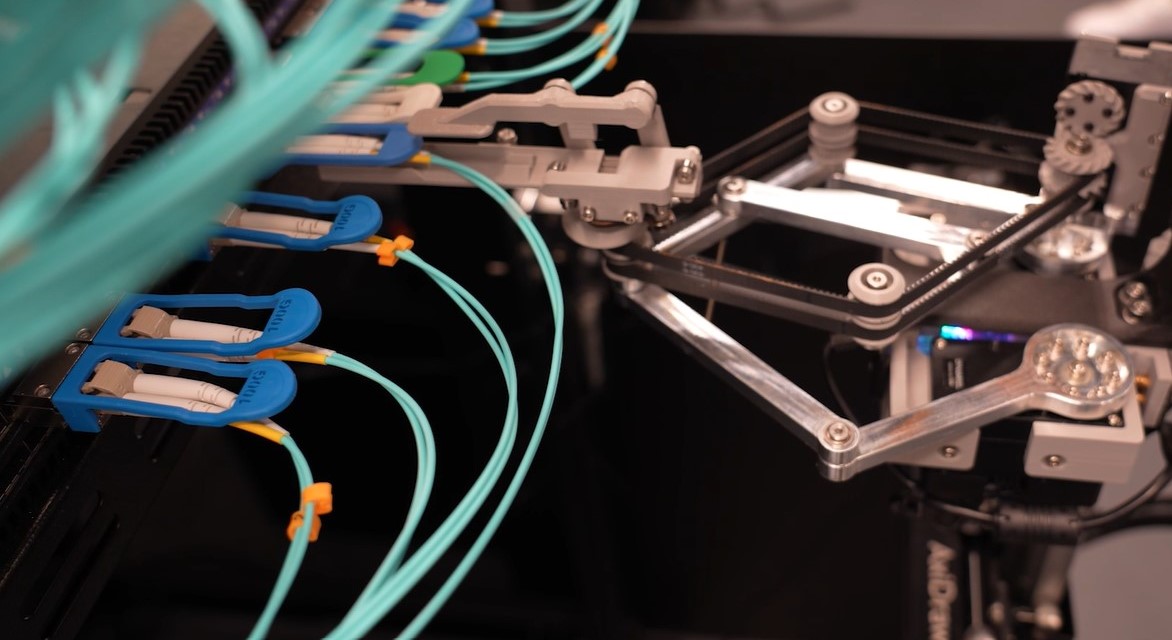
Publications May 1 Robust Optical Transceiver Manipulation in Cluttered Cable Environments Using 3D Scene Understanding and Planning